CIS 2210 - Database Management and Design

Chapter 11: Database Performance Tuning and Query Optimization

Objectives:

This lesson discusses material from chapter 11. Objectives important to this lesson:

1. Performance tuning
   
2. How queries are processed
   
3. How indexes affect queries
   
4. Query optimizer
   
5. Writing better SQL code
   
6. Tuning queries and the DBMS
   

Concepts:

Chapter 11

Performance Tuning

The chapter begins by telling us that textbooks often skip this topic. It is hard to demonstrate the benefit of efficient code with a small database. Classroom databases are typically small, so they don't provide a good case for fine tuning your SQL commands. In the real world, database tables can be very large, creating a need for code that runs faster.

On page 516, we see a template for an SQL query: The user creates the query. The client software sends the query, the server software receives and performs the query, and the server software send the result to the client that asked for it. We could add a step to include the client receiving the result and presenting it to the requester. The text mentions, in a side note, that there are things that will affect the speed of this process that are outside the scope of this text.  Some of them are listed in the table on page 517. Since these hardware, software, and network concerns are not things we can address in the classroom, the author will only discuss things we can do relating to SQL and to the database.

We can tune performance in two places, on the client and on the server. Tuning on the client will be mainly writing better SQL commands, which the author refers to as SQL performance tuning. Tuning on the server will be called DBMS performance tuning. The author does not outline what that will entail.

The author begins the next section with a look at the parts of a DBMS.

• files - As you know, tables are stored in files. A file can contain more than one table. Storage space for them is allocated on a storage device when a database is created. In a simple environment, files grow as needed. In a complex environment, such as Oracle, storage space may need to be expanded as files grow large. This expansion can be in predetermined increments called extents. As the information behind that link will show you, there are other database systems that use this concept as well, such as MS SQL. An extent has an advantage: it is an allocation of contiguous (sequential) memory addresses on a storage device. This makes access to files stored in this address range faster than access to files stored in discontiguous blocks.
• spaces - This disk space is allocated for a particular kind of files, such as a database or part of one, and it can be called a table space or a file group. There may be one for the entire database, or one for each kind of file, such as tables, indexes, user files, and temporary storage which works like a swap file.
• data cache/buffer cache - This is space that is allocated in RAM to allow very fast access to the most recently used data. The idea is that data you just worked with may be the data you will need again in a moment. This can be data you have just pulled from a disk, or changed data you have not yet stored on a disk. Regardless, the DBMS must put data into RAM before it can be used, and while it is in RAM, it can be read again faster than it was read from the disk. Disk read and write operations are bottlenecks that need to be managed. This is made more important on page 519, where the text reminds us of something we should know: it may take 5 to 70 nanoseconds to access RAM, and 5 to 15 milliseconds to access a disk. That's 5 to 79 billionths of a second, versus 5 to 15 thousandths of a second. Accessing RAM is not just faster, it is about a million times faster. A human may not notice the difference for a small file, but the difference adds up when there are many large files.
  
• input/output requests - The text reminds us that to read data from a disk or to write data to any device, the DBMS must interface with the operating system through system calls. These requests are affected by the actual memory block size used by the device in question.
• listener - Like any daemon on a server, this process waits for a request for a service it knows about. It watches for requests from the user(s), and routes those requests to other server processes.
• user - This is a process that stands for an actual system user or session. (A single human user may have multiple sessions at the same time.) It is the human user's avatar in the DBMS.
  
• scheduler - As we discussed in chapter 10, the scheduler process organizes requests from users.
  
• lock manager - The process that manages locking and unlocking data.
  
• optimizer - The process that met in chapter 10 that looks for the best, most efficient way to run all requests.
  

On page 520, the text revisits optimization, and proposes two ways to look at it. The first way is to order tasks so that the system takes the least amount of time to process them. The second way is to organize tasks so we have the lowest number of reads from, and writes to, disks. Reads and writes are dependably time consuming. The text presents a complex set of three perspectives from which to view such optimization:

• automatic or manual - An automatic optimization is chosen by the DBMS. A manual one is chosen by the programmer/user.
• run time (dynamic) or compile time (static) - An optimization method may be chosen at the time a query is run. If so, it is a dynamic method. If a query is embedded in a program that is compiled (perhaps written in one of the C variants), the optimization method may be chosen at that time, instead of when the query actually runs. That makes the method a static method.
  
• statistically based or rule based - A statistically based method relies on measurements of the system, such as number of files or records, number of tables, number of users with rights, and so on. These statistics change over time. They can be generated dynamically or manually. A rule based method, on the other hand, is based on general rules set by the user or a DBA.
  

The text gives us the impression that the statistical method is best by presenting a discussion of statistics gathered either automatically or by a command from a DBA. These methods are not mutually exclusive. The text states that Oracle, MySQL, SQL Server, and DB2 automatically track statistics, but they each have command to generate them as well. In MySQL, the command to get statistics on a table is ANALYZE TABLE tablename.

The text recommends that you regenerate statistics often for database objects that change often.

How Queries Are Processed

The text explains that the database processes a query in three phases, each of which has separate steps:

1. Parsing - Analyze the command and make a plan to execute it.
1. check the syntax
2. check object names in the data dictionary
   
3. check necessary rights for execution in the data dictionary
4. recompose the query to as needed to make it more atomic
   
5. recompose the query as needed to optimize execution
6. create an optimized plan for reading the data
   
2. Execution - Carry out the plan made in the Parsing phase.
1. execute the file access steps
2. add locks to files as needed
3. pull data from files
4. put data in data cache (in RAM)
   
3. Fetching - Carry out the verb sections of the actual SQL instructions, and present the results to the requester.
   

Note that the steps above are mostly hidden from the user unless an error is encountered. If there are no errors, the first ten steps may go by with little delay. The text points out that the result may be handed to the user in pages that represent the capacity of the data cache to hold sections of the result. In cases like this, it may be best to send the result to a file that may be examined more easily.

The text discusses five areas in queries can encounter processing bottlenecks:

• CPU - The text lists several problems that may cause the CPU utilization to be too high. Note that the CPU speed is only one of them. Make sure you review the others: low RAM, a bad driver, a rogue process,
  
• RAM - More RAM improves almost every computer process. It lowers the amount of swapping between RAM and cache space on disks, and speed up access to data that does not need to be swapped.
  
• Hard disk - Hard disk speed and access time affect disk swap time. So does available free space on the hard drive
  
• Network - Network transfer rates affect data flowing across a network, whether wired or wireless. Communication with a server across a network will never be as fast as using a server on the same machine as the client.
  
• Application code - The text includes the design of a database in this category. Bad design will slow down response time as will bad code in an application.
  

How Indexes Affect Queries

The text discusses the importance of having indexes for your tables. Page 526 illustrates using an index based on the State field in a customer table to find all the customers who live Florida. This is an example of an index file that you would have to create, since it is not the primary key for this table. Using the index, the DBMS quickly finds the row numbers of records in the table that match the search, and it pulls just those records into the temporary table used for the result. The text tells us that this method is faster than searching for those records in a full table search, which we would have to do if the index file did not exist, or if the index file was out of date. That is a key point for index files: to be useful, they have to be current.

The text further explains that the DBMS will automatically use an index file for a search on a field that has an index file. This is not an argument for indexing every field. The overhead for maintaining those index files would be substantial. It is better to analyze your transaction logs, and create indexes for popular searches. The text introduces a new idea: data sparsity, which is a measure of the number of different values found in a field. A field that has only two possible values has low data sparsity: lots of records may have either value. A field that has many possible values has high data sparsity: there are probably few examples of each value. In the example given of low sparsity, male or female, the use of an index on that field would not be much better than doing a search on the full table. In the example given of high sparsity, there will be relatively few cases of any particular birthdate. Indexing on that field may save search time.

The text lists three data structures on page 527 that are used to create indexes:

• hash index - This method actually seems to be taking a longer approach. The field being indexed is translated into a set of hash values. As you may know, no hash should ever be the same as another unless the material put through the hash function was the same material. This is one reason hash values are often used to prove authenticity of downloaded data. In this method, the hashes are sorted in the index table, and each points to the particular row in the table that its data came from. The text points out that this method is only good for exact matches, since a hash bears no similarity to the data used to create it.
  
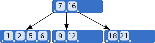
• B-tree index - The text tells us that this is the most common structure used in database indexes. It is quite simple, once you understand the idea, which is discussed more fully on this github page than in our text.
  
  
  
  
  
  In the example above, the tree allows for quick searches. The first layer tests the search value as being 7 or 16. If it is one of those, we use the pointer associated with the correct value. If not, is it less than 7, greater than 16, or between those values? Each answer takes us to a different block in another layer with more possible values. In a larger tree, we would have more values in the first layer, each of them leading to another set of values if the sought for value is not one of the values in the first layer. The illustration does not show that each match will point to a particular row in the actual data table. The text remarks that this structure works best when there are relatively few rows containing any particular value, but there are many possible values. This is called having high cardinality.
  
• bitmap index - The text recommends this structure when you expect to have lots of rows and only a few different values, and only a few concurrent searches. Having only a few possible values is called having low cardinality. This lesson from Oracle explains that a B-tree index can be a much larger file than the original table, but a bitmap index can be much smaller, so that structure is an advantage if storage space is an issue.
  

Query Optimizer

This takes us to a choice that will be made for us by software. Which kind of optimizer method should be used? The text describes two ways an optimizer might work:

• rule-based optimizer - Each action a query might take, like doing a full table scan or an index scan, has a rule for how much it "costs". The costs of each action involved in a query are added up, and the option with the lowest cost is chosen. The rules work on fixed costs, so this method is less flexible than the next one.
  
• cost-based optimizer - This method also uses costs, but it may rate the cost of an action higher or lower that the method above, based on statistics about the database objects, available RAM, I/O calls, and more. This is a more dynamic method that will vary with the hardware, the software, and the database in use.
  

Writing Better SQL Code

The text recommends writing better SQL commands to make their performance better. Although it should always be your goal to write better code, regardless of the language, the text presents two cautions:

• The optimizer in your DBMS may change your code, no matter how good you think it is.
• Recommendations for optimizing code will be different from one DBMS (brand) to another, and even from one version to another.
  

We are encouraged to write better code because it can make a difference. The optimizer works from general rules, but the person writing a command can know specific things about the data files that can make that command work better with that specific database.

The text gives us four situations in which an index file is likely to be used automatically (assuming it exists):

• If your query's WHERE or HAVING clause has only one column reference, and that column has been indexed.
• If your query's GROUP BY or ORDER BY clause has only one column reference, and that column has been indexed.
• If your query uses a MAX or MIN function on an indexed column.
• If your indexed column has high data sparsity. (Remember: high sparsity means lots of different values, and relatively few repetitions.
  

The text introduces a new phrase: high index selectivity. The phrase means that you have indexed on a field that is very likely to appear as a criterion in a search. (Latin root word: one criterion, two criteria.) There is no point to creating an index on a column that no one cares about. The author's point is that we should anticipate the kind of searches that will be done in a database, and create indexes that support the actual work. The text makes some recommendations about making index files:

• Searches run faster if there is an index for each field used as a single attribute in restrictive clauses: WHERE, HAVING, ORDER BY, GROUP BY.
• Indexes add little or no value when there is low sparsity in the indexed field, and when there are few records in the table.
• Primary keys automatically get index files made for them. Use that by making sure to note primary and foreign keys in table declarations.
• If you are running joins that are not natural joins, consider creating indexes for the fields used in the joins.
• Older DBMS systems did not use indexes when the indexed field was used in a function in the SQL command. Newer ones may allow function-based indexes. The text gives us an example of a function-based index: YEAR(INV_DATE) would mean to extract the year portion of the date a row-item entered inventory. The author suggests making an index on this function. This seems like an odd example, since this function would lead to a collection of data with little sparsity. It appears that the author believes that we may as well try.
  

The text continues with some observations about conditional expressions, which are usually the parts of the command that restrict the rows that are returned:

The text makes a special note that Oracle does not follow the evaluation rules referenced in the table above.

On page 534, the text continues the discussion, but with a different point of view. Often you will begin an IT project with the end somewhat defined, but the beginning and middle will be unknown. This happens when the customer knows what kind of results the system will have to produce, but they are counting on you to figure out the inputs and the processing that will match the sort of output they need. That's the position you are in at the top of page 535, where the author begins a series of steps that will lead to a database answer.

1. What columns (from which tables) will you need to produce your outputs? And what processes will you have to perform on the data to get the desire information? The author suggests that you consider both of these questions together. You will also want to know about any system information you will need, such as time and date. And you should consider what built-in functions you can use, and what processing you will have to figure out on your own.
2. The author suggests that you should identify tables that hold the information you need. I think this will have to be done in conjunction with the first step, otherwise how could you identify columns? A better point he makes in this step is to pull data from as few tables as possible to reduce the complexity of your queries.
3. Most data you pull will come from natural joins, but step three is here to consider outer joins. Make notes, and come back if necessary.
4. Think about the WHERE and HAVING clauses. What will be the filters on your selections? Do you need to run a series of queries, saving the results as you go?
5. Think about the proper display of information. Will you need to use ORDER BY and/or GROUP BY clauses?
   

On page 536, the text turns to tuning the performance of the DBMS itself. This is something you will not be able to do if you are a user of the system, and not an administrator. It begins with a list of DBMS features that an administrator can change:

The topic changes a bit to discuss hardware changes that would improve server performance:

• RAM - The server can avoid frequent disk access if it is possible to load the entire database in RAM. Eventually, the changed database must be written to long term storage.
• SSD drives (I/O accelerators) - If your data is stored on an SSD drive, access is faster than on traditional hard drives.
• RAID - The use of RAID systems can provide faster access, although it would be slower than the two methods above. It also provides some protection against drive failure, depending on the RAID level in use. Several kinds of RAID exist to provide for redundant storage of data or to provide for a means to recover lost data. The text discusses three types. Follow the link below to a nice summary of RAID level features not listed in these notes, as well as helpful animations to show how they work. Note that RAID 0 does not provide fault tolerance, the ability to survive a device failure. It only decreases the time required to save or read a file.

  RAID levels and features:

  • RAID 0: Disk striping - writes to multiple disks, does not provide fault tolerance. Performance is increased, because each successive block of data in a stream is written to the next device in the array. Failure of one device will affect all data. This will provide a performance enhancement by striping data across multiple disks. This will not improve fault tolerance, it will in fact decrease fault tolerance.
  • RAID 1: Mirroring and Duplexing - provides fault tolerance by writing the same data to two drives. Two mirrored drives use the same controller card. Two duplexed drives each have their own controller card. Aside from that difference, mirroring and duplexing are the same: Two drives are set up so that each is a copy of the other. If one fails, the other is available.
  • RAID 5: Parity saved separately from data - Provides fault tolerance by a different method. Data is striped across several drives, but parity data for each stripe is saved on a drive that does not hold data for that stripe. Workstations cannot use this method. It is only supported by server operating systems.
  • RAID 6: An improvement on RAID 5; it uses another parity block to make it possible to continue if two drives are lost.
  • RAID 1+0: Striping and Mirroring - uses a striped array like RAID 0, but mirrors the striped array onto another array, kind of like RAID 1. Expensive, but recommended.
• Disk contention - It is possible to affect performance by using a storage scheme that should reduce the incidence of multiple requests for the same part of the database. The text recommends this scheme:
  • system table space - to hold data dictionary tables, which are accessed frequently
  • user data table space - create separate spaces for each application, or for each job type assigned to your users (not for each user)
  • index table space - to hold the indexes used by each application or for each user group as needed
  • temporary table space - again, separate spaces for each application or group of users
  • rollback segment table space - to be used when transactions must be rolled back/recovered
  • high usage table space - for tables that are used the most often

The text offers several other organization based ideas, but these are enough for this section.

The chapter ends with an analysis of an example query in an Oracle environment.